What do a doctor and a car mechanic have in common? Both cure/repair a broken instance, but before they can do so they need to make a proper diagnosis which can only be done if sufficient relevant data is available. The doctor will combine the patients’ medical history with laboratory results and results from specific medical tests while the car mechanic will look at the maintenance history and read out the on-board computer. For both, their senses – especially eyes and ears – also provide indispensable information.
What is new to both the doctor and the car mechanic is that the amount of data they have available from their respective sources is increasing rapidly. Due to proper digitization and access to medical records the doctor has instant access to your whole medical history, including what you’ve forgotten yourself or what you’re not mentioning now. After the consultation the doctor sends a blood sample to a medical lab for analysis and a single such request typically has boxes ticked for dozens of different measurements. The biggest provider of data to the doctor comes from the field of medical imaging: the latest magnetic resonance imaging (MRI) scanners don’t just output images that resemble those from your 1994 webcam anymore, but in one session make tens to hundreds of images up to 3 megapixel in size (Stucht et al., 2015). If the doctor is looking at the patients tissue samples under an electron microscope he or she will hopefully data hungry, because these images you can now get in a whopping 64 megapixel (TVIPS, Gauting, Germany).
Meanwhile, the car mechanic has connected a handheld device to your car via the standard On Board Diagnostics (ODB) connector to receive a full overview of everything that has been measured by the car. The amount of data this generates has grown with the increasing complexity of our cars.
For both the doctor and the car mechanic the amount of available data has increased to the point that for a single human being – no matter how experienced in their field – it becomes a big challenge to filter out the irrelevant data, and get a grasp on all possible combinations of the relevant features that could lead to a proper diagnosis. This diagnostic data that is crucial to diagnose the condition of a system can be taken care of by a data scientist in a way that it supports the field expert in their decision making.
Our doctor and car mechanic aren’t the only ones who work with diagnostic data. Think about the enormous amount of logging data originating from IT-systems like programs, websites, or mobile apps. There are a multitude of reasons something can go wrong, and more often than not more time is spent on interpreting these logs and finding the cause of the problem than on actually solving it. These days more and more electronics have become “smart” and “connected”, and with that also comes an increasing amount of diagnostic data.
In the next section we will discuss the main ways of how a data scientist supports field experts into diagnosis by building what we will call a data-driven diagnostic system. Thereafter we will present some state of the art solutions.
How we deal with diagnostic data
Like with many other practices in the field of data science the distinction between supervised and unsupervised learning is crucial to explain how we deal with diagnostic data.
Supervised learning
In supervised learning our dataset on which we want to build a data-driven diagnostic system not only contains symptoms for all our sick patients (or cars for that matter) but also contains the diagnosis based on the expertise of one or, preferably, more experts. If we use multiple experts the probability of mistakes is reduced, and better data quality will result in better preforming models. The task for the data-scientist is to create a model based on this data that will then be able to give a reliable diagnosis given a certain set of symptoms.
The following table shows an example of the data available. As I’m not a medical practitioner I decided not to use existing symptoms and diagnoses so stuck to an abstract example.

The table shows four patients for whom there has already been a diagnosis. Patient X on the other hand should receive a diagnosis by our data-driven system. How does this work exactly? A naive approach would be to look only at the most similar cases: Patient X has exactly the same set of symptoms as patient 2 so it would make sense to give them the same diagnosis (B), right? Maybe Symptom 3 isn’t very specific for the kinds of diseases we’re studying here, and when we ignore that variable patient X also matches with patient 4 which had diagnosis A. There is however this patient 1 who also had diagnosis A but did have Symptom 2, so that doesn’t fit either. Furthermore, in practice we won’t just have data available showing the presence or absence of a few symptoms, but a very wide table with all possible medical measurements and checks. As the number of possible combinations of symptoms or values on these measurements will grow exponentially we’ll soon have more possible clinical pictures than we’ll ever have patients making it near impossible to find good matches. As you can see our naive attempt to learn by matching won’t give a good solution in this case. Check out the book The master algorithm: How the quest for the ultimate learning machine will remake our world (Domingos, 2015) for a more elaborate explanation on different paradigms in machine learning and why they (don’t) work.
A better approach would be the construction of a decision tree that converts all (relevant) symptoms into nodes that split into two or more paths which flow to other symptom nodes or to a diagnosis. The following figure shows how a decision tree for this example could look:

Figure 1: Decision tree to diagnose diseases based on the presence of certain symptoms.
In our example you could have come up with this tree yourself, but for large datasets proper tree-generating algorithms are used as the data easily surpasses the capacity for a human to do this properly. These algorithms will put the most important variables (symptoms, measurements, …) – those that are most capable to distinguish between different diagnoses – earlier in the decision tree and then further split increasingly similar clinical pictures. Keep in mind that a reasonably sided dataset is required to generate a reliable decision tree as otherwise the tree will perform poorly when using it to make new classifications. In contrast to the previous technique, variables that are not relevant at some point in the decision making process will automatically not present there. In medical practice diagnosing based on these kinds of models is part of the clinical decision support systems that guide medical practitioners into taking the best decision.
Decision trees are very popular for these kinds of classification problems, especially as they are easily understood which allows the users not only to come to the predicted classification (i.e. diagnosis) but also to get insights from them. Other techniques in supervised learning are often a bit more difficult to understand but can have other qualities like improved classification accuracy. Examples are support vector machines and neural networks.
Unsupervised learning
In the previous section we could learn from cases that had already been diagnosed in the past but this is not always the case. In unsupervised learning we cover those techniques that deal with an unknown target or diagnosis. Imagine you’re studying unknown pathogens under a microscope. For each instance you write down a list of properties. How do you know if you’re (most likely) dealing with a single kind of pathogen or multiple kinds that look alike at first? We can’t use the techniques from supervised learning here because we don’t have a target variable (the kind of pathogen), while in the previous case there already existed cases where the target was known.
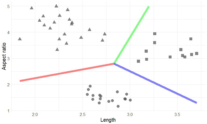
Let’s take a look at two of the variables you noted down for each of the pathogens: length and aspect ratio. Length (in ?m) of the longest edge of the pathogen, and aspect ratio is the ratio between the shortest and longest edge. We draw a scatter plot where each individual pathogen is represented as a single data-point with length on the horizontal axis and aspect ratio on the vertical axis:

Figure 2: 50 data points devised into three clusters based on two variables.
It’s immediately clear in this example that we can define different groups or clusters: The small but elongated ones (triangles), the medium sized more or less round ones (dots), and the bigger ones with average aspect ratio (rectangles). The colored lines represent boundaries between the clusters. The clustering technique can’t tell if each group is a completely different kind of pathogen or not, but it does give the researcher an interesting suggestion what to look for. In this example it is easy to spot the clusters with the naked eye, but if we take more variables into account that becomes tough (three-dimensional scatter plots are possible but are already harder to read). This is where the techniques from unsupervised learning come into play: they can handle large numbers of variables and will tell you which ones are relevant. Depending on the kind of problem you’ll choose another kind of clustering technique; popular ones include hierarchical clustering, K-means, and DBSCAN.
Examples of data science applied on diagnostic data
Detection and classification in images
As mentioned earlier the medical sector heavily relies on high detailed imaging. With the growth in size of this data, the chances that important information is available but overlooked increase. Researchers are therefor looking at ways to automatically detect and count specific targets like cancerous cells (e.g. Cruz-Roa et al. 2017).
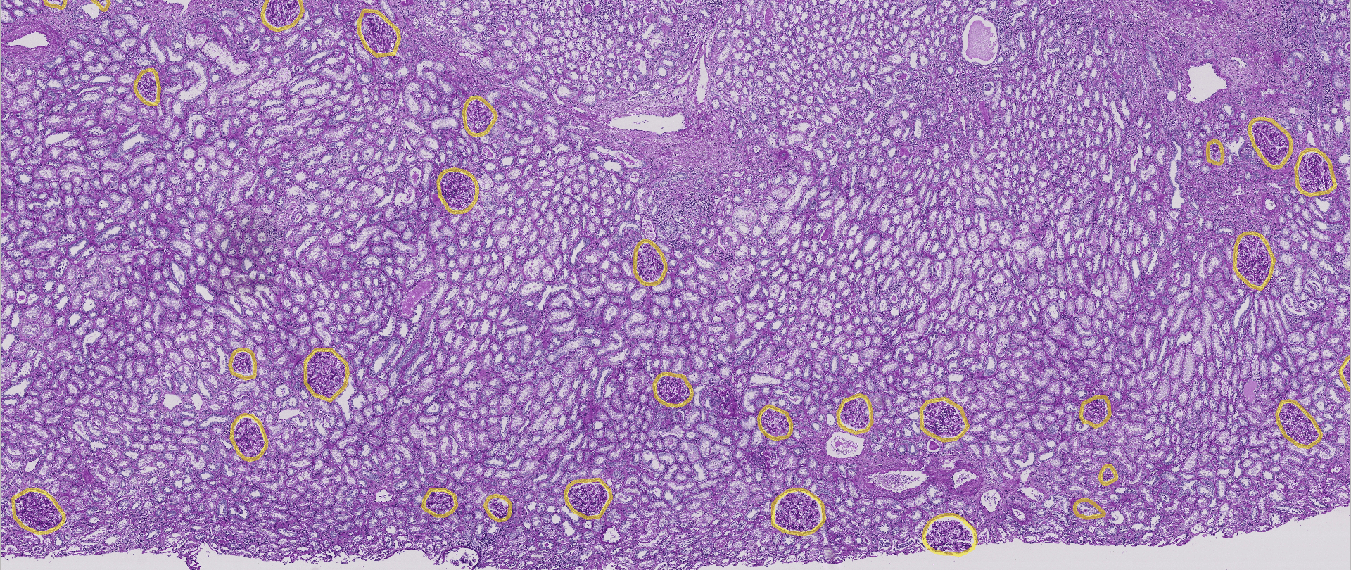
A recent data-science competition by Kaggle (2020) challenged data-scientists to do a similar task: Trying to detect the glomeruli (a type of networks of small blood vessels) in a human kidney. In order to train their models the participants got access to a large collection of high-resolution images and a data set containing the exact position and shape of the glomeruli. Their models would then be evaluated by applying their model on a new set of images (as is the usual course of events in machine learning). Note that this is an example of supervised learning: experts first had to manually annotate where the glomeruli are in order to create the data sets. The following picture shows part of one of the images with the glomeruli marked with a yellow circle:

Figure 3: Glomeruli on the human kidney.
Apart from detecting certain things in images (where is it?) you often also want to classify it (what is it?). In practice these two tasks are often combined in a single model that detects different kinds of objects (e.g. different kinds of cells) and also assigns them to their respective category. This article is not meant to be technical so I’m not going in on the actual methodology of detection and classification in images. If you’re interested you should check out convolutional neural networks which is the main power-tool for these kinds of problems.
Another field where you can see the use of detection and classification in images as a tool for diagnosis is manufacturing. The sooner in the production process a defective instance is detected the less it will cost you in the end. To avoid having more defects you want to diagnose what went wrong with this instance so proper action can be taken to avoid having more defective products. The next figure visualizes this. The “patient” is now a teddy bear instead of the human we’ve mainly been talking about, but from the data-scientists point of view we’re dealing with the exact same challenge.

Figure 4: Defect detection (left) and classification (right) on a production line.
Predictive maintenance
Prevention is always better than cure, no matter if we’re talking about the health of a human being, the state of your car, or something bigger like the correct working of an offshore drilling rig. Predictive maintenance studies techniques to optimize maintenance in a way that intervention happens before an issue occurs in order to avoid it from happening. It is related to diagnosing as it also looks for the link between symptoms and disease, but it differs in that it tries to intervene before the disease breaks through. As you might expect, predictive maintenance relies heavily on the availability of data and techniques from data-science.
Predictive maintenance in humans is, for example, the use of the so-called “activity trackers”: smart watches or other wearable technology that monitors your activity and/or other vitals and encourages you to keep up a healthy lifestyle. This contrasts with planned maintenance like a yearly medical checkup or corrective maintenance which is an intervention when something already broke (i.e. you’re sick).
Let’s take a closer look at what predictive maintenance for an offshore drilling rig would mean. You don’t want to exaggerate with planned maintenance due to the big cost, but having to do corrective maintenance is certainly to be avoided due to the enormous impact that would have (ecological, or financial, for example). Apart from oil, this rig also receives a large amount of data: sensors monitor pressure and flow in all the pipes, properties of the pumped up oil get monitored, and outside influences on your oil rig like the wind and sea waves are constantly recorded. Again we’re looking at an amount of data a human cannot properly interpret in its raw form. Data-science is capable of determining which variables are relevant and goes way deeper into the data by also looking at complex interactions between multiple variables, and derivatives such as increases in the speed with which pressure builds up in a pipe. The predictive maintenance system will be able to alert you to take actions before something occurs. It will warn you to replace a part before that part fails, just because the system predicts there is a decent probability of that part failing soon. By knowing in advance you avoid sudden shutdown and can replace the part in a much more cost friendly matter.
Conclusion
Let’s summarize what we’ve discussed:
Diagnostics isn’t the exclusive field of medical practitioners. Every complex system, whether it is as small as a single computer chip or as big as an oil rig, might at some point get “sick” and will present multiple symptoms that can aide the diagnosis.
Data is crucial for proper diagnosis and therefore indirectly responsible for the selection of the proper cure.
The amount of data that is available and relevant to achieve this proper diagnosis is most often too big to be properly processed without the use of machine learning and other techniques from data science. These techniques are used to build a data-driven diagnostic system.
If you wonder what the use of diagnostic data could mean for your company, let us know and we’ll discuss the possible solutions.
References
Cruz-Roa, A., Gilmore, H., Basavanhally, A. et al. (2017) Accurate and reproducible invasive breast cancer detection in whole-slide images: A Deep Learning approach for quantifying tumor extent. Sci Rep 7, 46450.
Domingos, P. (2015). The master algorithm: How the quest for the ultimate learning machine will remake our world. Basic Books.
Kaggle (2020). HuBMAP – Hacking the Kidney.https://www.kaggle.com/c/hubmap-kidney-segmentation
Stucht, D., Danishad, K. A., Schulze, P., Godenschweger, F., Zaitsev, M., & Speck, O. (2015). Highest Resolution In Vivo Human Brain MRI Using Prospective Motion Correction. PloS one, 10(7).
Any questions? Don’t hesitate to contact me: joris.pieters@keyrus.com
