Blog post

How to solve every problem in the world: Explaining the power of genetic solvers

Joris Pieters

What if - hear me out - there was a way of solving every problem in the world? Ok, maybe not all of the world's problems, but all problems related to optimization. Optimization refers to the practice of finding the optimal set of values for certain parameters so that we can get to (or close to) an optimal solution. This field of study is called Operations Research. Here are some examples of optimization problems:

• You're producing different kinds of dog food. Every week you obtain certain quantities of different ingredients. Each kind of dog food you produce has a unique composition. The cheaper ones (where you will typically also get a lower margin) have a recipe comprising of a lot of grains and some cheaper meats while the more expensive ones are mainly made from lamb and beef and smaller amounts of grains. Your goal is too choose how many bags you'll produce of each kind that week so that you'll maximize your profit while keeping in mind that you'll have to stick to the available quantities of each ingredient.

• You're working in a large production facility that exists of multiple adjacent units. Not all units are constantly manned; this depends on what is being produced at any given moment. A manned units has an extra cost due to lightning, heating, and supervision. Your task is to figure out a production schedule so that the number of units in use simultaneously is minimized while still meeting the production quota.

Note that in the first example we want to maximize profit while the second one is focused on minimizing costs. This is what we call the objective. The objective can be anything, and in most cases it is some kind of value we want to either maximize of minimize.

Both the examples are what we call discrete problems which means that the answer will be in integer numbers. In the production facility example each unit is either in use or not at a certain point: e.g. even if it's running at half capacity you'll still need to provide full lightning, heating, and supervision. The dog food mixing case is similar in that we want to end with fixed numbers of bags for each composition (as our customer won't be buying half a bag). If we did the bagging ourselves but provided the dog food in bulk however, it would be a continuous problem.

Both examples also contain constraints which set limits to what solutions are feasible. For the dog food this is the amount of every available ingredient. In the other example it is that you have to meet the production quota, otherwise the solution would be so naive as to just shut down the whole plant as that would minimize the costs. In more technical texts you'll see constraints mentioned as subject to.

Now that you've got a better understanding of what optimization is we'll explain how they are typically "solved". Thereafter we'll dive into genetic solvers that form a framework for all kinds of problems that are out of range of the classic methods.

We'll not get too technical in this article; that might be something for a next one. The goal in this text is to get you interested in the amazing world of solvers and how this often overlooked discipline in data-science can help your company.

How to solve these problems?

The madman's way

A possible way to find an optimum (i.e. minimum or maximum depending on your objective) would be to try out every possible solution. For continuous problems it's not even worth considering this as the number of possible solutions is infinite. You could try this for a discrete problem but unless we're talking about really small numbers, the number of possible solutions grows astronomically and therefore becomes practically impossible to compute.

Just to give you a feeling about this: you've got a problem that requires you to decide which of the six production lines in your factory need to run at a certain point. Each of the lines has a different capacity, fixed running cost, variable running cost, and other properties making it a rather complex problem (i.e. it's not just a matter of how many lines we run, but which ones specifically). One possibility would be to run zero (which will certainly not lead to a feasible solution as you actually need to produce something). There are six possible combinations to run a single line, 15 to run two, 20 to run half of them, again 15 to run four, six to run five of them, and finally there is of course a single way to run them all. That's a total of 64 possible solutions. Doubling the number of lines will not double the number of possible solutions here. It will square this number: with 12 lines you have 4096 possible solutions! What about 100 lines? Well, imagine every possible solution would take the size of a grain of sand; you would need over a billion earth-size spheres to contain all those possible solutions! It would be pretty clear that "trying every possible solution" would not be a very useful strategy.

The somewhat smarter way

Instead of trying all possible solutions you might be more tempted to use your own experience and intelligence to come up with a set of rules to solve the problem. Such an approach is called a heuristic. A possible heuristic for the dog food problem could look like this:

1. Select the recipe wherefore the bags of dog food have the highest profit margin.

2. Manufacture that type of dog food until one of the ingredients runs out.

3. Select the next most profitable type of dog food for which you still have ingredients left ... and so on.

Although this might often give a decent solution it will probably not be the best one. As the more profitable type of dog food contains more meat (and less grain) you'll probably get stuck with an excessive amount of grain that is of no use (as even the cheapest kind will need some meat). Therefore the optimal solution will probably be one where a bit less of the meat-rich variety is made.

A heuristic you probably use quite often is finding the shortest route between two locations (cities, ...). Humans using traditional maps as well as navigational apps on your phone or in your car make use of heuristics to figure out what is (probably) the best route.

A special heuristic is the treatment of a discrete problem as a continuous one as these are typically more easily solved. If we go back to the dog food example that would mean ignoring the fact that we can't end up with non-whole bags and rounding the results to down to integer numbers for every type of dog food we offer. However, this is often not the optimal solution, though it must be said that with large numbers (i.e. hundreds or thousands of bags) the difference between this approach and the best discrete solution might be negligible.

The mathematician's way

Many problems and accompanying constraints can be expressed as mathematical equations. The optimization then really becomes a matter of finding the minimum or maximum of a function within the boundaries set by said constraints.

I promised not to get technical so let's limit ourselves to an extremely simple example: you're hosting a stand that sells variety of home bottled fruit juice. These are the two compositions that you offer:

If you have 10 liters of apple juice available and 4 liters of blueberry juice, what is the maximum total amount of drinks we could make with above recipes? The completely naive method of trying every possible solution is obviously out of the question now as we have a continuous problem (i.e. the number of liters we make from each mix doesn't have to be a whole number).

Now let's try a very simplistic heuristic: start by making one drink until you run out of ingredients for it and see if you could still make some more of the other drink. From Mix 1 we can make 12.5 liter using all 10 liters of apple juice and 2.5 liters of blueberry juice. Note that the ratio is correct for Mix 1, namely four times more apple than blueberry. You've used all your apple juice but still have 1.5 liter of blueberry juice left. Sadly no recipe we're offering can be made with only blueberry juice. Conversely, if we started with Mix 2, which has a much higher concentration of the more scarce blueberry juice we would only be able to create 12 liter using 8l apple and the full 4l blueberry juice. 2l of apple juice stays unused this way. We now know there is a lower limit of 12.5 liter mixed drink we can create, and we have at least some suspicion that making some of both the mixes might result in the biggest total amount of mixed drinks. But how much will we create? Will we reach 13 liters, 13.5 maybe? And what will be the proper ratios?

Let's first introduce some proper notation by putting the objective and constraints into mathematical expressions. The objective is to maximize the total amount of the two mixed drinks which we'll call X and Y, so we write "Maximize X + Y". The first constraint is that the total amount of apple juice must not be greater than 10 liters. As a liter of Mix 1 (X) is made of 80% apple juice while this is two third of a liter for Mix 2 (Y) we can say that 4/5 X + 2/3 Y can not be more than 10 (liters). Similarly a fifth of X plus a third of Y must not exceed 4 (available liters of blueberry juice). Additionally we add two extra constraints: both X and Y must not be negative as it is quite obviously impossible to generate a negative amount of mixed juice. Together we write this down as follows:

Now there exists a nice mathematical way to find for which values of X and Y their sum is maximized given said constraints, but - as I promised not to get too technical - let's stick with the graphical way to answer this question. Let's draw a graph with the horizontal axis expressing the amount of Mix 1 to make, and the amount of Mix 2 to make on the vertical axis. Every point (x, y) you would put on this graph corresponds with a certain amount of both mixed drinks. The further to the top right of the graph the higher the total amount of mixed drinks. Now let's add the constraints to the graph: the first two constraints take the form of a triangle (red and blue respectively). A point within this triangle complies to the constraint. The purple area thus complies with both constraints. The two so called non-negativity constraints are also present here though less explicitly: we take these into account by not letting our red and blue area extend under the horizontal, or left, of the vertical axis. The purple area where all constraints are met is also called the feasible region.

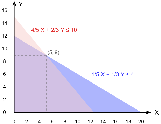
Now it's just a matter of finding which point (x, y) is within the areas defined by the constraints where the sum is the highest possible. As we already know the optimal solution will not be to make either only Mix 1 or Mix 2 this point can be found by looking for the "kink" in the feasible region. This seems to be located at point (5, 9) which tells us we must make 5 liters of Mix 1 and 9 liters of Mix 2 for a total of 14 liters which is way above the 12.5 liters our overly simplistic heuristic gave us! Let's check if this solution is indeed feasible:

Mix 1 requires 80% apple juice, so for the assigned five liters of Mix 1 we'll need four liters of apple juice. For Mix 2, two thirds of our nine liters needs to be apple juice; combined we get a required amount of ten liters which is exactly what we have at our disposal.

Similarly for blueberry juice the sum corresponds to the available amount. Obviously, with more ingredients and more complicated recipes this problem would become a bit more difficult and might also result in optimal solutions where not all ingredients are used completely. This example should however suffice to give you a taste of the capabilities of mathematical solving (admittedly we used a "graphical way" instead of the purely mathematical way as it's easier to understand but they are inherently equivalent).

Is mathematical solving then the answer to all problems? No, if they can be used we should use them but there are some limitations:

1. To represent your problem and constraints as mathematical equations you might need a mathematician.

2. Some parts of your problem or constraints will be terribly difficult to put into an equation.

3. Having an equation does not mean that we can actually solve it mathematically! (e.g. certain fifth or higher order polynomials)

The versatile alternative: the genetic solver

Inspiration from biology

Genetic solvers follow a totally different approach inspired by the way evolution works. When two individuals of a species breed they share their DNA creating new individuals with traits found in Mom or Dad, but also some new ones that result from how the exact way the DNA got mixed. If certain traits are beneficial for the survival and breeding of the offspring there is a higher probability this trait gets passed through to the next generation. This is a rather slow process because a lot of randomness is involved, but after many generations it can lead to substantial changes resulting in the situation where you are reading this text instead of sitting in a tree nibbling juicy leaves.

DNA exists of chains of four molecules, basically making it a quarternary numeral system, therefor containing double the information per bit compared to the binary system (only two different values, normally expressed as 0 and 1) that a computer works with. Though the way information is encoded is slightly different, we can use the principles from biology to allow potential solutions of a problem to "evolve" towards an optimum and thus using it as a solver. Instead of strands of DNA we'll talk about arrays of bits when we move away from the biological world.

There are multiple mechanisms for how two strands of DNA (i.e. one from each parent) combine to a new one (the offspring). The most commonly known mechanism is called crossover where part of the strand from one parent is replaced by the corresponding part of the other partner.

The use case

Let's take a real-world example of a problem we would like to solve with a genetic algorithm. Our example is a case of a vehicle routing problem: You have to deliver pallets 47 pallets of goods to your clients. You have to make sure that each pallet gets delivered and of course you want to do that for the minimal total cost. To reach that goal you have the following trucks available:

There are three sizes of trucks, e.g. we have 12 small ones with a capacity of two pallets and so on. Every size of truck has both a cost per km (mainly fuel, maintenance, and depreciation), and a cost per hour (mainly cost related to the driver). To calculate route costs we'll use OpenStreetMaps (OSM) to provide us the distances and driving times between the depot and all delivery locations as well as between all delivery locations mutually (of course this is done via an API and not manually; but that's a story for another time). As the OSM driving time predictions are rather optimistic, certainly for the medium and large trucks we added a correction factor "Relative speed" by which we divide the driving time of OSM to obtain a more realistic estimation.

We assume that every truck will only do a single tour per day and the cost only results from distance and time driving. Actually we'll use a lot of simplifications, not because genetic algorithms can't handle complex scenario's but because we want to keep this article fun to read.

A quick multiplication of truck amounts and capacity shows that we have a daily capacity of 55 pallets which is enough for the 47 that are waiting for delivery.

Our - fictional - depot is located in a small town called Strombeek-Bever just north of Brussels. This place also happens to be the home of Keyrus Belgium, but that is purely a coincidence. The 47 pallets need to go to 47 different delivery locations spread across Belgium.

A naive attempt

If you're familiar with similar problems in the field of Operations Research you might think this is an example of a simple assignment problem where you have to assign a set of workers to a set of tasks. In those problems however the tasks are basically independent of each other (apart from the fact that if one worker gets a certain task assigned you can't assign it to another one anymore). In our example however there is an extreme interdependence between the tasks. For example, if you need to deliver a pallet in Ghent that can be done relatively cheaply if you also have to deliver one in Bruges (as Ghent is more or less on the way between our depot and Bruges), while the same pallet would result in a much higher additional cost if it was put in a truck on its way to Liège (the complete opposite direction).

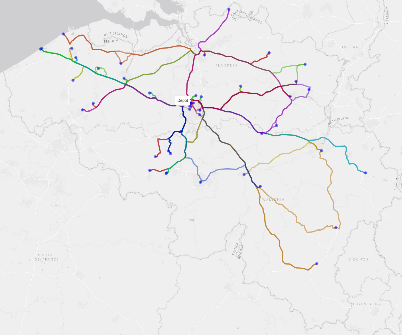
Let's start very naively by putting all 47 pallets in a random order in one of 55 slots. The pallet in the first slots will be handled by the first truck, and so on. Each pallet has its specific destination. Eight slots will remain empty.

We load the trucks and they start their route. At this point both the assignment of pallets (and thus destination) to trucks as well as the order in which a truck delivers its pallets is completely random and thus absolutely un-optimized. We calculated the total cost of this operation using distance- and duration tables obtained with OSM in combination with the above table with cost/km and cost/hour; the result is €6776. Additionally your drivers will also be pretty annoyed with your complete lack of efficiency and consider you a poor manager. The following image shows the (badly) assigned routes with each color representing one of our trucks:

First improvement: optimization per truck

The first optimization we're going to do is to change the order of delivery for each truck separately. This problem where you have to find the least costly way to visit a certain set of locations and returning back to the first one (in our case the depot) is called the travelling salesman problem (TSP) which is probably one of the more famous problems in Operations Research. Though traditionally explained in terms of minimizing the total distance, you can just as easily use any kind of cost metric, as in our example. Though simple to explain it's a hard problem compute-wise as the only way to make 100% sure you've got the best solution is to check all possibilities and this number of possibilities grows exponentially with the number of locations to visit. Luckily for us however this problem is so well studied that very good algorithms and accompanying software packages exist so that we don't have to figure out this part ourselves. After letting a TSP-solver loose on each of the trucks we reduce the cost to €5581 and get the following solution:

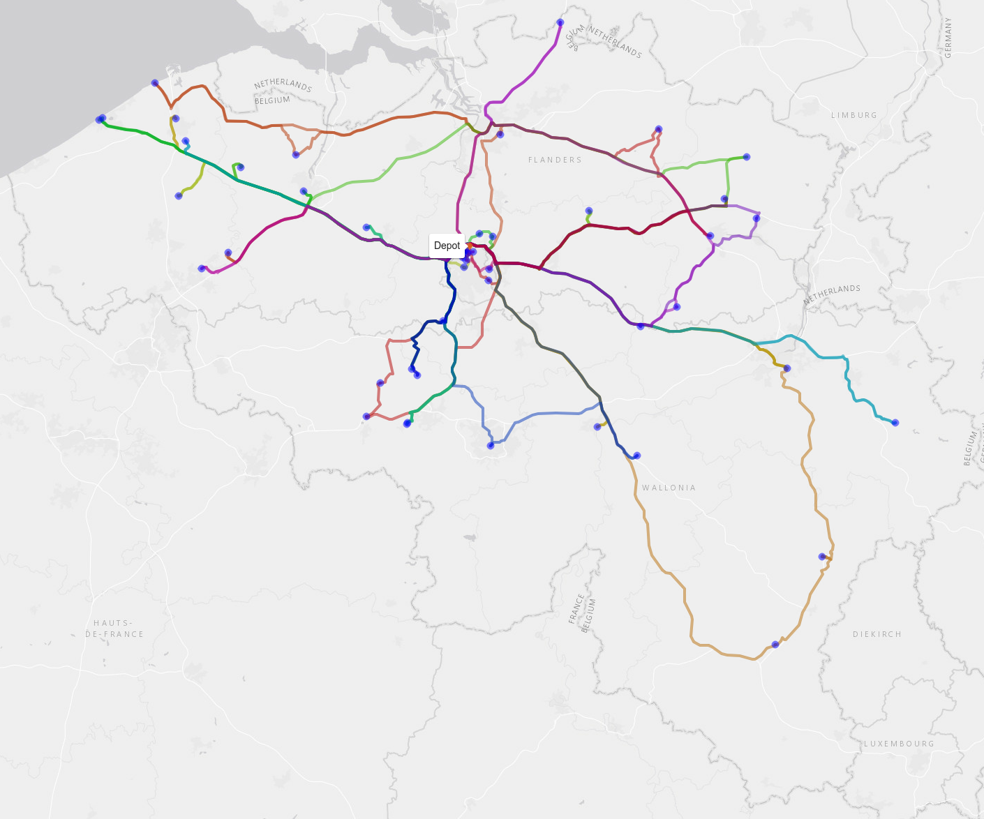
This is an improvement, but only optimizing per truck will still result in many suboptimal solutions like two trucks going to the same two cities both to deliver one pallet each instead of having one serving the two clients in one city and the other taking care of the other city.

Time to go genetic

In order to use a genetic algorithm to assign the pallets in an optimal way we need to figure out a way to represent this as a binary array (i.e. a series of zero's and ones). This is often the most difficult part when it comes to programming these kinds of solvers. One way to approach the problem here is to start from the line of 55 slots we mentioned earlier where each slot contains either one of the pallets or is empty (as we only have 47 to deliver) and find a way to encode each possible order in a binary way. As the order of the pallets within each truck does not matter we can reduce the number of necessary bits further.

Once we've figured out how to represent this as an array of zero's and ones (for completeness, genetic solvers exist that deal with decimal numbers too, but that also is a story for another time) we can offload the heavy work to a library specialized in genetic optimization. There are a few parameters to choose, but they are easy to understand given the similarity with the biological counterpart. An important one is the population size, where smaller populations will obviously get processed faster but will more easily get stuck in a local optimum and thus not improve further. The most tricky parameter you'll have to decide on is how long - in terms of "generations" - you'll keep the algorithm running. Remember that a genetic algorithm is not guaranteed to provide the optimal solution, nor will it be able to tell if an optimal solution has been reached. There are however a few indicators that show you can stop "breeding", for example if no improvements are observed for multiple generations.

In practice we often start with a very simple example where we can find a (near-)optimal solution in another way (for example by trying out all possibilities). If our genetic algorithm converges to that solution we have a good indication it will also perform well with real problems. From these small examples we can also calculate an average expected cost per pallet delivery. As we scale up this cost is expected to lower as the probability increases of having multiple delivery locations close together that can be served by the same truck. Another common strategy while tuning and evaluating the genetic algorithm would be to have it run a few times with a different (random) first generation of "parents". If totally different starting populations reach a similar (or similarly good) result that is a strong indication your genetic algorithm is performing well.

A library for solving genetic algorithms typically also allows you to "choose" part of the "genes" of your first generation. If you can think of some easy to implement heuristics that already give a significant improvement over randomly chosen solutions it's really advised to add those as it will help the genetic algorithm a great deal to find a good solution faster. Additionally you should keep the results of your solver because even though you might have a different task each day (e.g. other delivery locations) there will be recurring patterns. The knowledge obtained from previously solved cases can help to find better start heuristics.

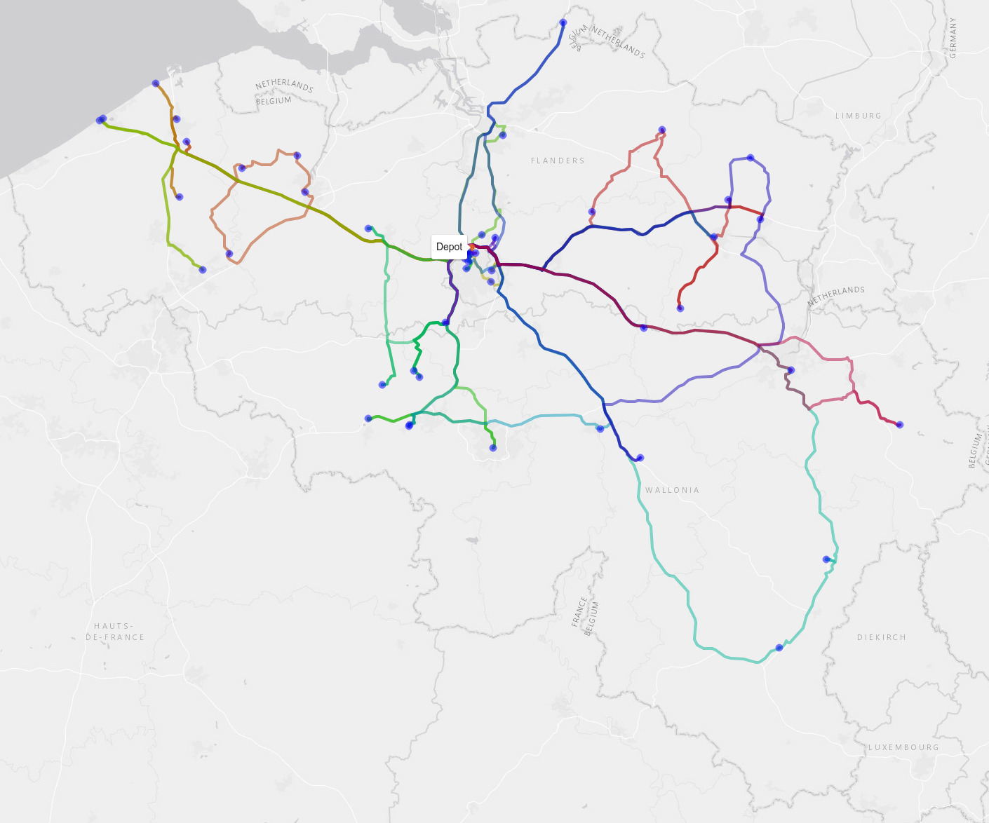
We applied this on our example (using the "genalg" package in R) and let it run for a few generations until no further improvements seem to happen. It turned out that the best solution we found would cost us €3836, which is nearly half of our original (though admittedly rather stupid) initial estimate:

Potential extensions

We focused on the way a genetic algorithm is capable of providing a good solution for a not so simple problem. In practice however our case study was actually still very much an oversimplification of reality. This choice was made to keep the article easy to read, but I hope by now you realize that the power of genetic algorithms is that you could basically pass any kind of function that calculates your costs or profit (or whatever you want to optimize). Here are some potential additions that we could easily implement:

• Different package sizes and packing optimization.

• Multiple packages at same destination.

• Order of packages in the truck.

• Addition of loading and unloading times.

• Addition of waiting times if too many trucks want to load at the same moment.

• Limit number of different trucks to use in a day (i.e. less drivers needed).

• Multiple trips per day per truck.

• And much more...

Conclusion

Every company has to deal with optimization problems from time to time but often sub-optimal solutions are chosen as they are good enough and improvements are considered too hard. I hope that while reading this article you have came to the enlightening realization that there might be a whole lot of "low-hanging fruit" at your business waiting to be optimized, maybe with the use of a genetic algorithm.

I admit that this article did not provide you with enough technical knowledge to start implementing one of these amazing optimization techniques yourself as the required skills and knowledge are a bit bigger than what I can cover with a blog post. Luckily though there are people at Keyrus who can help you with that!

If you've got any questions, don't hesitate to contact the author via joris.pieters@keyrus.com