A collaboration between Keyrus Belgium and the Department of Environment and Spatial Development of the regional Government of Flanders.
In this article we'll present how we created yearly maps of soil cover for the whole area of Flanders at a detailed level. We achieved this by combining existing sources of known reasons behind soil cover with a three-dimensional convolutional neural network applied on aerial photos to fill in the unknown parts. The improved monitoring we achieve here is a crucial tool to follow up on measures taken to assert the land is used in an environmentally sustainable way.
Background & challenge
Soil cover refers to the permanent covering of soil surface making it impermeable for water. Common sources of soil cover are of course buildings and roads, but also smaller less noticeable constructions like patios, driveways, or sheds.
The reduced amount of water infiltration due to increased soil cover leads to an increased amount of precipitation that won't have the chance to be absorbed by the soil. The consequences hereof are twofold: On the one hand the soil gets dryer which will increase heat issues in urban areas, reduce the amount of CO2 storage of plants and trees, and reduce the biodiversity. On the other hand there is also an increased risk of flooding in some areas when all the precipitation ends up in an overloaded sewage system.
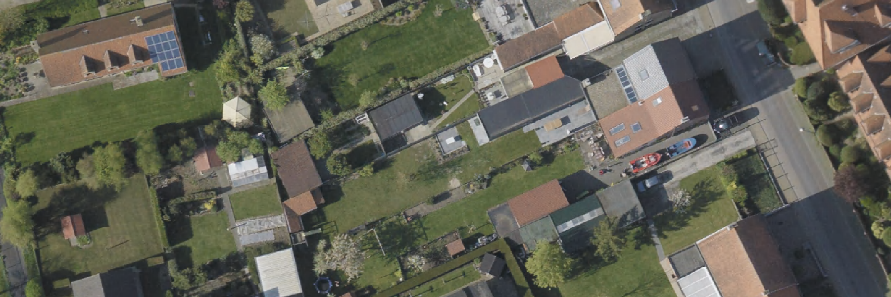
With around 15%, Flanders (Belgium) is one of the areas in the world with the highest degree of soil cover and this percentage is increasing at a rate of approximately half a percentage-point every three years (Pieters et al., 2021). Because of the adverse effects of high levels of soil cover which the Flemish people are already experiencing now, combined with the perspective of a worsened situation if no appropriate action is taken, the Flemish government has made it a priority to revert this dangerous evolution.
To be able to get better insights into the current evolution, as well as to monitor the effects of measures that will be taken to combat the increase of soil cover in Flanders, the government was in need of a high quality measuring instrument. It was decided that a yearly area-covering map with a resolution of 1m² showing which square meters of soil are covered would be required. The maps would also be created retrospectively, starting from 2013. Keyrus was happy to assist the Department of Environment and Spatial Development of the regional Government of Flanders who got assigned the task to create these maps. In the rest of this article we will mainly focus on technical achievements wherefore Keyrus provided a helping hand. For the more general context we refer to the official paper (Cockx et al., 2022; in Dutch).
Approach
There were two stages in this project: firstly we created soil cover maps from aerial photographs with the help of artificial intelligence, and secondly we combined this with other data sources so that every square meter would get assigned a value of either uncovered or covered based on the most reliable source of data available for that specific pixel.
Detection of soil cover using artificial intelligence
Every year aerial photographs covering the whole of Flanders are made at a resolution where every pixel corresponds to an area of 25 cm by 25 cm. As Flanders measures 13.624km², that corresponds to nearly 220 billion pixels per year. That's more pixels than Elon Musk lost dollars in 2022.
Over 1000 images of 1024x768 pixels were cut out of aerial images between 2012 and 2020. In total this corresponds with a total area of approximately 50km². Each of these was presented using a Wacom Cintiq 12wx drawing tablet where a well-instructed person coloured the pieces of the image containing soil cover.

From each of these images we cut six 512x512 pixel (as we cut with 256 pixel overlap) and also create three rotations (90, 180, and 270 degrees) to maximize the total amount of available material to over 24.000 images.
70% of the 512x512 pixel images were assigned to the training set; the remaining were kept for validation. Images from the same original picture were always either all in the training set or all in the validation set.
The model used is U-Net, a three-dimensional convolutional neural network originally aimed at semantic segmentation in medical images (Ronneberger, Fischer, and Brox, 2015). Initial testing and comparison with other semantic segmentation models taught us that U-Net didn't bother if it had to detect soil cover rather than glioblastoma, so we went with it. Eventually we reached an accuracy of 96.8% on the validation set. The implementation of the model was done using TensorFlow (Adabi et al. 2015).
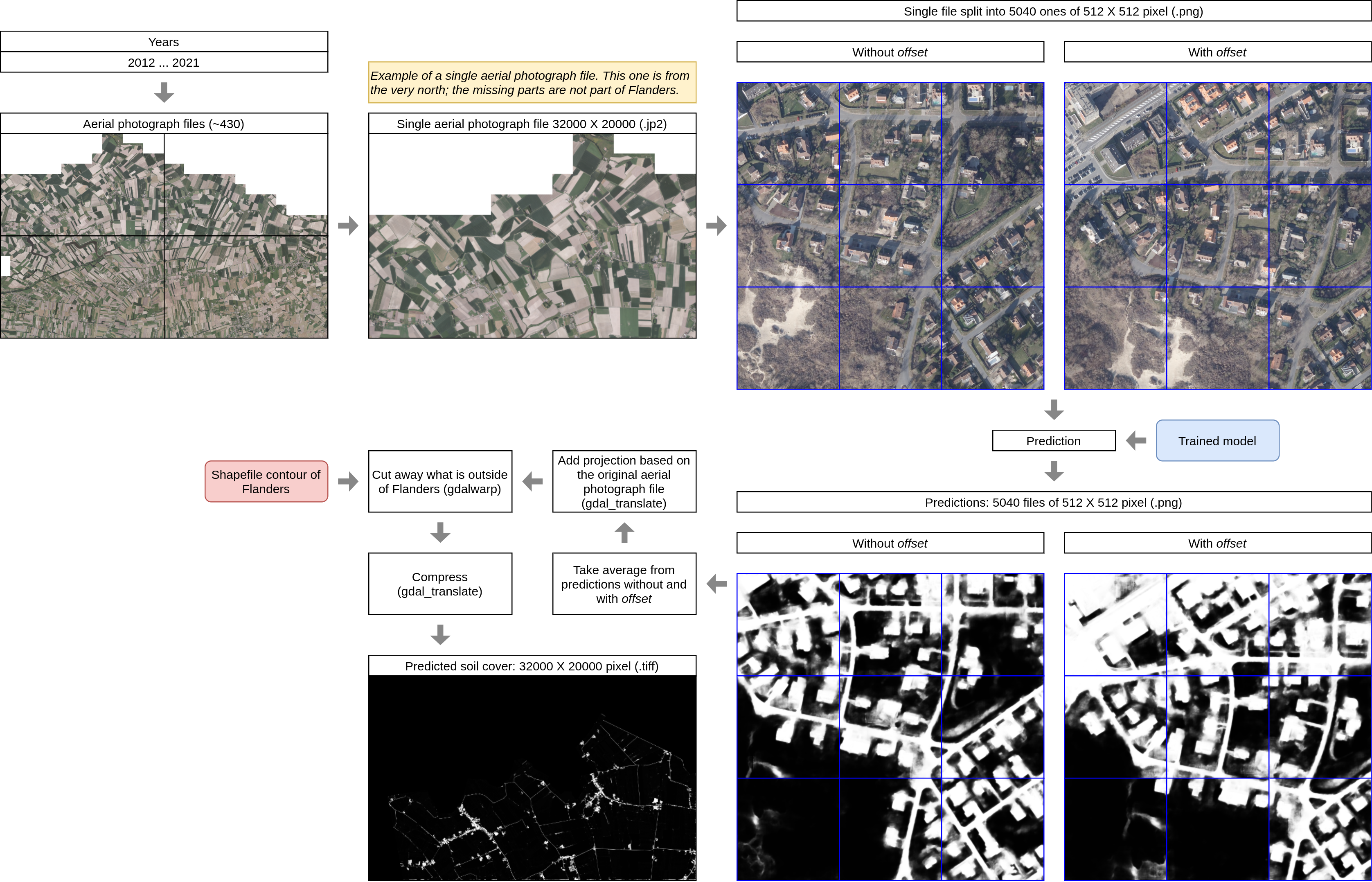
The next step was to apply the trained model on the aerial photographs of the whole of Flanders for all years from 2012 up until 2021 (the latter had just become available by then). The aerial photographs are available in about 430 files of 32000x20000 pixels. For each of them, we cut them into 512x512 pixel files. Because the model tended to be less accurate at the edges of these images we actually did this a second time where we cut similar sized pictures out of the original image a second time, but now with a 256 pixel offset. Therefore, for every pixel, the soil cover was actually predicted twice and we then averaged the results to generate an even more reliable result. After that the original projection was copied to the soil cover map (i.e. make it an image with geospatial reference again), and for those at the edges we cut away parts not belonging to Flanders. The following image shows the different steps in this process:
All code to generate the predicted soil cover files was written in Python and heavily relied on the gdal library for geospatial processing.
Preparation of other data sources
Listing all other sources of data here would lead us too far away from the essence so for now we'll keep it high-level. All of these sources exist in the form of vector maps of different types of objects for which we can either say for sure that there is soil cover (e.g. buildings) or that there certainly isn't any soil cover (e.g. waterways). For all of these the situation at any point in time can be accessed, so it was possible to obtain yearly extracts corresponding with the years for which we want to generate soil cover maps.
A special case were vector maps of roadways, for which the polygon vectors are actually way wider than the actual road and therefore also contained some non-covered parts. Within most of those polygons there exist line vectors demarcating between covered (actual road) and non-covered parts (verge), as well as line vectors indicating the approximate middle of the road. Each of these vectors is shown in the following image:
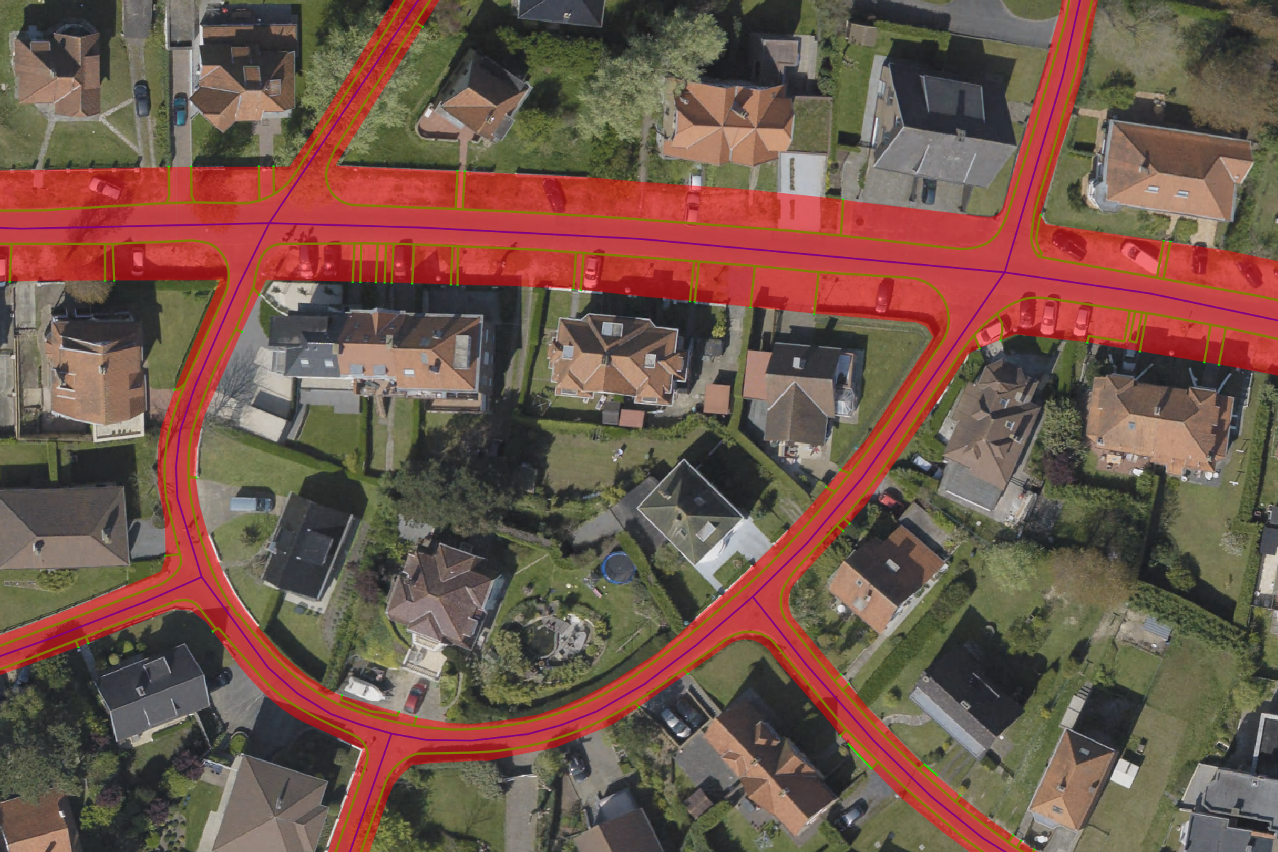
In order to create polygons containing only areas where soil cover is certain we had to come up with a custom algorithm that could make the separation based on the available vectors. Simply put, this algorithm looked which areas were on a roadway, between demarcations, and got intersected by a middle of a road. In other words, corresponding to the above image, keep only the red parts that are delineated by green lines and having a blue line within.
The code for this part - as well as for the next one - was written in R.
Combining all the data to definite soil cover maps
The soil cover maps created with artificial intelligence were converted from a resolution of 25 cm by 25 cm to 1 meter by 1 meter and thereafter each cell was converted to a binary value indicating if the soil is covered or not. Here we added an additional correction against inaccuracies: Manual comparison of these maps with the aerial photographs revealed that false positives (a pixel indicating soil cover where there wasn't any) and false negatives (a pixel indicating no cover where it should) were typically not consistent over time (i.e. they would show up on the map in one year but not in the one previous or thereafter). Furthermore actual change (addition or removal of soil cover at a specific point) is typically not a fluctuating process: once a certain pixel has changed it is less likely to return to its previous state (e.g. you don't pour concrete just to break it out a year later). It was therefore decided to correct pixels that had only changed for a single year as mistakes by the algorithm. Manual checks confirmed that this decision would increase the overall accuracy. The disadvantage of this method is however that you need to have the prior results of the surrounding years. This explains why the first soil cover map will be for the year following the year for which we started to apply the artificial intelligence model (i.e. 2012), as well as why the map for the last year will always be considered a temporary one which will - one year later - be replaced by a definitive one whereon this correction could be made.
All vector maps were converted to raster maps with a resolution of 1 meter by 1 meter in correspondence with the artificial intelligence soil cover maps.
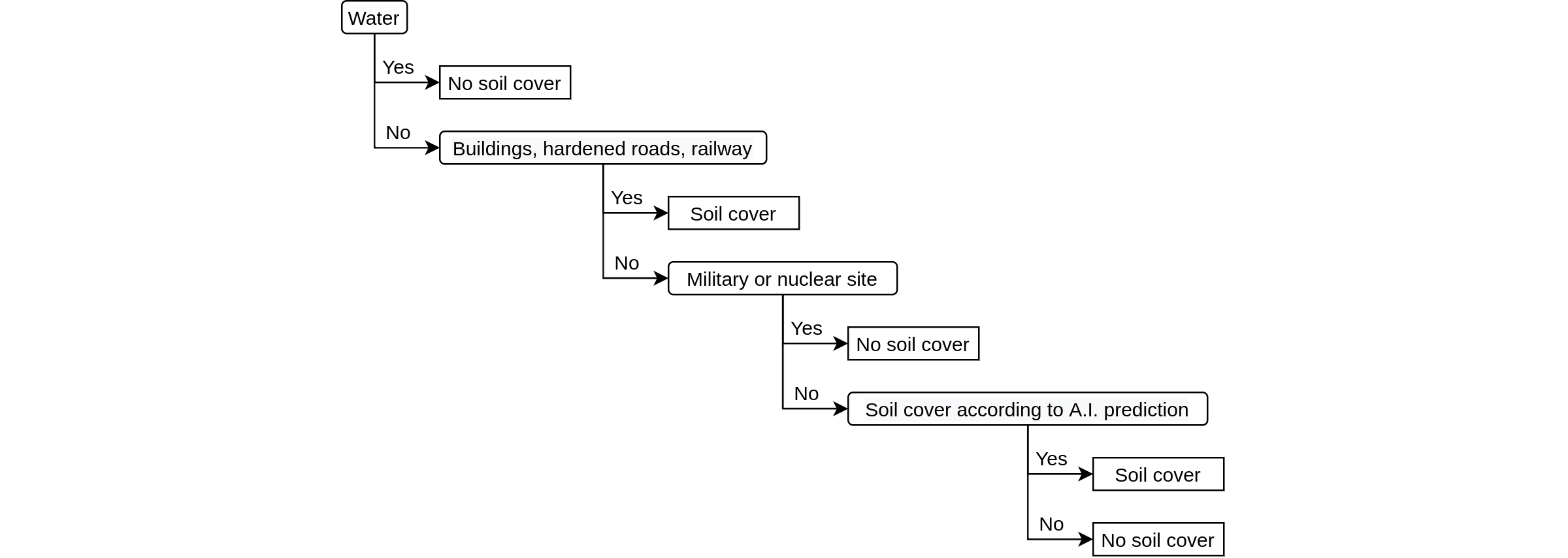
Finally we combined the different sources using a decision tree starting from the most reliable data sources. Not mentioned earlier are the military and nuclear sites: as they are blurred on the aerial photographs the artificial intelligence model could not be applied there and therefore raster cells in those areas wherefore we had no information from another source (buildings, roads, ...) were always categorized as "No soil cover".
Apart from the 1 meter by 1 meter binary maps (i.e. soil cover or not) we also created derivative 5 by 5 meter maps where each raster cell contains a values representing the percentage of soil cover, as these lower resolution maps are typically easier to work with.
Key results
Accuracy of the Soil Cover Maps was investigated by comparing the maps with manually labeled material. On a 1 meter level an accuracy of 97.8% was reached on average; for the 5 meter maps this was 98.0%. Not only was this a substantial improvement compared to the existing soil cover maps, the big win is the decrease of manual labor needed to create new maps in the future. From now on a new map will be released every year.
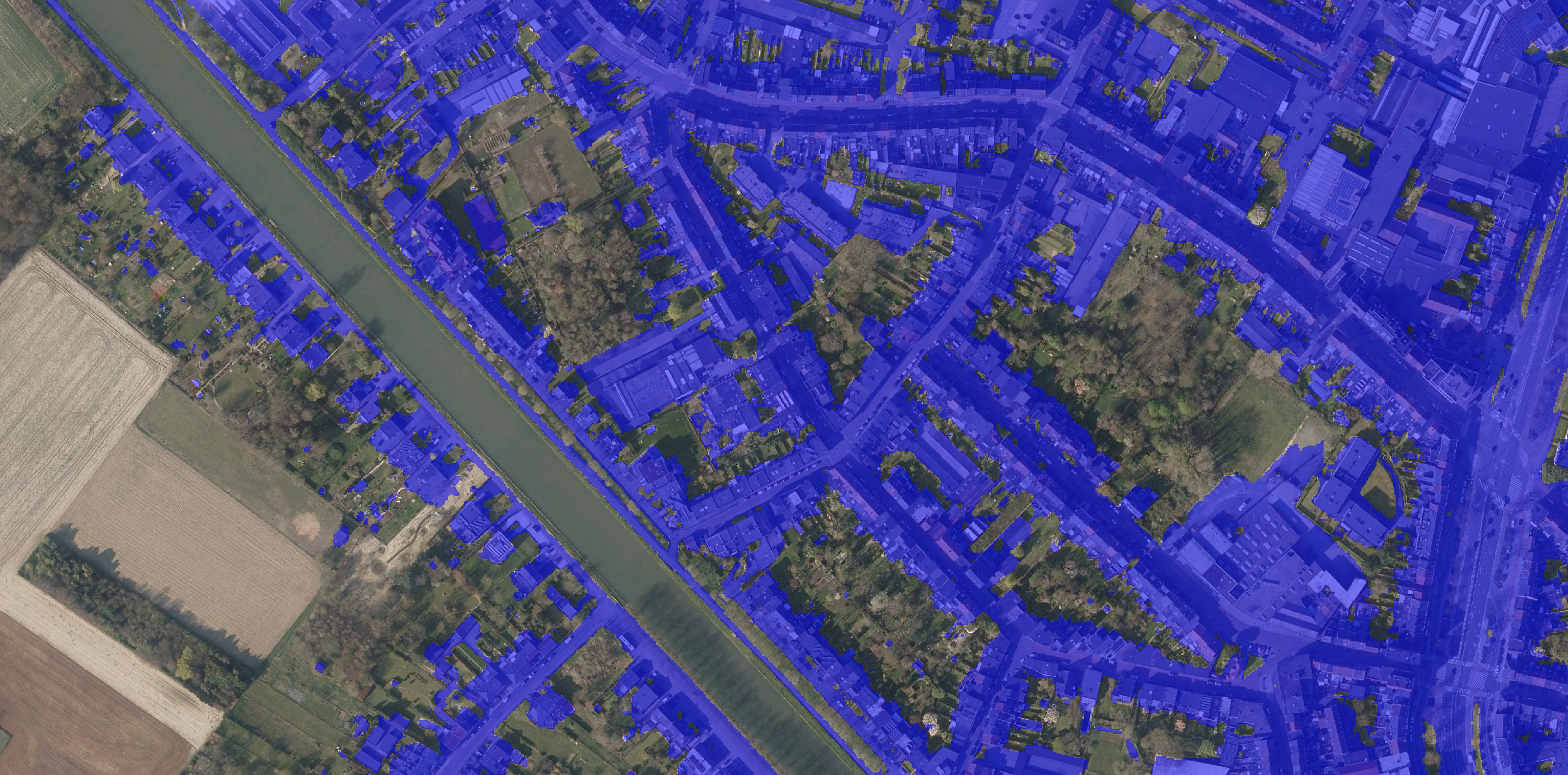
Between 2013 and 2021 we see a near linear increase in soil cover in Flanders of approximately half a percent point every three years, reaching around 15.5% in 2021. Measures are being introduced to limit the amount of new soil cover and to remove some of the existing soil cover. Thanks to this new instrument the Flemish government will now be able to quantify the impact of said measures relatively quickly and hopefully stop the current yearly increase.
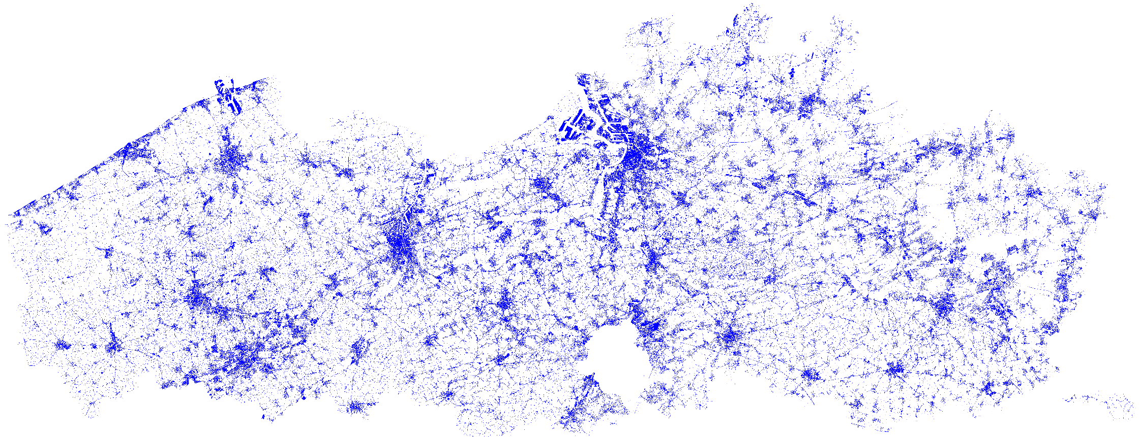
The official paper (Cockx et al., 2022) can be found here. The actual maps can be viewed online and downloaded on the website of the Flemish government (search for "JaarBAK").
If you've got any questions, don't hesitate to contact the author via joris.pieters@keyrus.com
References
Adabi, M., Agarwal, A., Barham, P., Brevdo, E., and Chen, Z. 2015. TensorFlow: Large-Scale Machine Learning on Heterogeneous Systems. https://www.tensorflow.org/.
Cockx, K., Pieters, J., Willems, P., and Vanacker, S. 2022. Jaarlijkse Bodemafdekkingskaart Vlaanderen: Technisch Rapport. Vlaams Planbureau voor Omgeving.
Pieters, J., Willems, P., Brems, W., Vanacker, S., and Pisman, A. 2021. Evolutie van Verharding En Ruimtebeslag in de Periode 2012-2015-2018. Vlaams Planbureau voor Omgeving.
Ronneberger, O., Fischer, P., and Brox, T. 2015. U-Net: Convolutional Networks for Biomedical Image Segmentation. arXiv:1505.04597.
