The Incentive behind the Vectorization of Old Maps
One of the ways to understand the evolution of roads over time is to digitalize them using the vectorization technique. The advantages are multiple and allow for urbanists to make better predictions for the future and explain the past transformation of a certain geographical area.
Manual interpretation is often needed to compare historic with current situations as the former old maps are not readily available in a vectorized format. These time-consuming operations could be done much more efficiently if the old data were available in a structured and searchable format.
Images versus vectors
Even when properly digitized, including the addition of the right projection parameters, comparing images of maps is typically a manual task if the information on the map is available only in the form of an image and not vectors. Vectors are basically just sets of numbers which are well suited for all kinds of mathematical operations. This makes them well usable to answer questions ranging from descriptive ones like the total length of roads per municipality, over analytical questions like explaining the evolution of roads in function of the land uses, up to predicting future road expansions.
The following image shows the difference: on the left is a (modern) map, on the right is a representation of the roads in vector format.
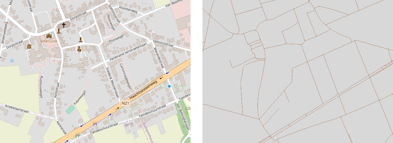
Figure 1: A map versus the vectors representing the roads
For modern maps we do have these vectors; the images are even generated based on these vectors. For old maps however we only have the images available. In this article we’ll describe how we generated vector maps for the roads in 1904, 1939, 1969, and 1989 on the territory of Flanders (Belgium) as part of an assignment of the Environment Department of the Flemish government.
Training a machine learning model to detect roads
Manually tracing all the roads on the old four maps would be a tedious and inefficient thing to do, so we decided to use machine learning instead. For each of the four years we selected 250 locations at random and cut out a piece of 1024 by 768 pixels. Each of these was then presented on a drawing tablet (Wacom) and data labelers were asked to trace the roads as accurately as possible.
The labeled images were cut into smaller ones, and fed to the “Roadnet” neural network which was originally made to detect roads on orthophotos. As the way maps are drawn has evolved over time the style was rather different, so we went for separate models for each of the four maps.
Once trained we applied the models to the whole territory of Flanders. To do this we first had to split the whole of Flanders into small images, apply the model to each of them, and paste them together again. Here an issue arose: while the models had really high accuracy overall, the predicted images often had artifacts at their edges where the model sometimes falsely assumed the edge of the images corresponded with a road. To solve this we applied the models again, but this time on pieces of the map that were horizontally and vertically shifted by 50%. In other words, pixels at the edge in one image would be in the center of a shifted image and vice versa. We then combined those predictions, and only pixels that were considered to be a road in both the unshifted as well as the shifted image were finally considered to be roads. The following image explains this:

Figure 2: Left: 2 by 2 predictions. Full blue pixels are correct predictions, hatched blue ones on the edges are false positives. The middle image is a shifted prediction corresponding with the area marked by the orange square in the left image. The right shows the result where only pixels predicted by both unshifted and shifted were kept.
A majority of artifacts were resolved this way but we were still kept with some small false positives. For example, railroads are drawn as alternating black and white pieces, and the white pieces were incorrectly classified as belonging to a road. Because roads typically connect at least on one side to each other these false positives could easily be identified with an algorithm as they have a limited size and are not connected to other pieces. Using contour-detection from the image processing library OpenCV we could identify separate pieces and remove those under a certain threshold.

Figure 3: Before and after removal of small artifacts (background shows the corresponding map for illustrative purposes only).
On the old road maps different colors were used for small and big roads. The data labelers had not made a distinction between these, but as the difference is rather pronounced, we made the distinction based on a simple algorithm that looked at the underlying average RGB-values.
Vectorizing and matching the vectors to current roads
At this point we had basically extracted all roads from the old road maps, but this result again was an image (though one with just two possible values per pixel, one for “road” and one for “no road”). Using the “AutoTrace” library we converted those into vectors.
At this point we had vectors that very well represented the roads on the old maps. To compare with the current situation of roads in Flanders we even had to a bit further: Even when a road was present both in the past as it is now the vectors would never align exactly due to inaccuracies on the old maps or because the middle of a road would be located slightly differently over all these years. The following image illustrates this with the vectors contained from the 1904 map in blue and the current roads (black). Most roads that were present back then still exist, but a lot of roads have been added:

Figure 4: Before matching, black lines are current roads, blue ones are those in 1904.
Because of the large number of additional roads, we have to be careful trying to match the old roads to the new ones as a general “best fit” method would not necessarily result in the proper result. We therefore based ourselves on the “iterative closest point” algorithm which is better suited for matching different sets of vectors. For those old roads where we did find a match (i.e. roads that have not disappeared over time) we replaced the vectors with those of the corresponding current road. This can be seen in the following image:
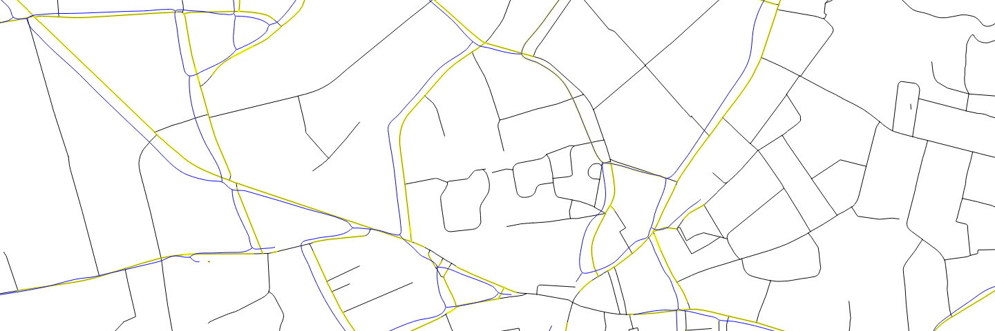
Figure 5: After matching, the corrections are shown in yellow.
Conclusion
For each of the four maps we reached an accuracy of over 98%, which is higher than what you often get when doing a similar task on pictures. These drawn maps did seem very well suited for the neural network we used. By creating vectorized versions of these old road maps we now have better material to study the evolution of roads in Flanders over time.
At least as impressive as the accuracy number is the visual result: below are two examples of the same area in 1904 and 1969 where we colored the detected roads (green for bigger roads, blue for the smaller ones).
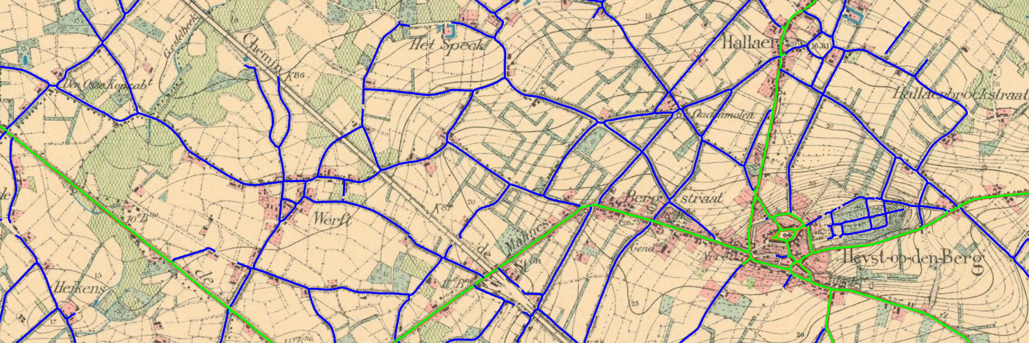
Figure 6: Detected roads: 1904
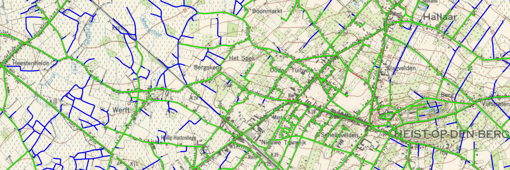
Figure 7: Detected roads: 1969
Thanks to this work it has now become much easier for analysts to investigate changes in the Flemish road network over time. Better understanding of past changes will assist making predictions of how the network will expand in the future, as well as guide policy makers in how to steer those into a desired direction like in the following sample applications:
Studying the evolution of the road network growth gives us the opportunity to estimate future nuisance resulting from traffic, like air- or noise pollution. This allows us to look for alternatives like the development of other roads or other modes of transportation to prevent the undesired side effects from traffic to reach undesirable levels. Meanwhile we can optimize the flow of traffic to make the most efficient use out of the public roads.
Urban sprawl – the development and growth around a city – can result in an increase in traffic related issues. Roads leading to and from the city might not have the capacity to handle the increased throughput, and the single-use zoning typical for these kinds of areas often results in an even faster increase in traffic compared to multi-use zoning where people rely less on their personal car. Additionally, the growth of towns and cities over time can result in them merging into a single urban area with degrees of human movement well beyond the capacity of what the roads were initially intended for. With the knowledge of the evolution of the road network over time that we now have it becomes possible to predict how the network will look like in the future if no actions are taken, thus identifying future issues and prevent them by responding appropriately.
To read more about the useful applications we refer to the “Ruimterapport 2021” of the Environment Department of the Flemish government: https://omgeving.vlaanderen.be/ruimterapport (in Dutch).
Questions? Contact the author Joris Pieters at joris.pieters@keyrus.com
